Choosing Priors in Bayesian Analysis: A Gentle Guide

After my talk at PyCon DE & PyData 2025 in Darmstadt — titled “Getting Started with Bayes in Engineering”, I had some great conversations with attendees who were curious, about the role of priors in Bayesian modeling. In other instances, I have also seen some skepticism on this topic.

It became clear to me that for many newcomers, the idea of “choosing a prior” feels confusing, subjective, or even unscientific. And I get it, I remember struggling with that too.

So I decided to write this blog post to walk through how I personally think about prior selection, and what has helped me make sense of it. This isn’t the only way to do it, of course, but it’s a practical, honest approach that balances intuition, data, and model behavior.

Along the way, we’ll use a real dataset (human heights and weights), build a few simple models in PyMC, and perform both prior and posterior predictive checks to see how our assumptions play out.

🔍 Note: The code in this post is adapted and extended from the PyMC documentation on predictive checks — which is a great reference if you want to go deeper.

Let’s get started by asking a simple question:
What kind of process do I believe generated the data I’m looking at?

Start with the data

Before we even get to choosing priors, we need to backup a bit and ask:

What kind of process do I believe created the observations I see?

This is your generative model, and is what determines your likelihood. It explains how your data came to be.

The likelihood is just a term for:

Given some unknown parameters, what’s the probability of observing the data I actually saw?

So how do you pick a likelihood?

Start by looking at the type of data you are modeling. That usually points to a small set of reasonable choices. Let’s look at a few examples:

If your data is a count (like the number of cars crossing a bridge each hour, or the number of people voting in an election), you might assume that the data generation process follows a Poisson distribution. Thus, your model might include a rate parameter: something that should be positive (can’t have a negative number of cars!).
If your data is a continuous measurement (like height, weight, or temperature), a suitable candidate to explain the data generation might be a Normal distribution. A model under this assumption might include a mean (any real number) and a spread (standard deviation or variance, which must be positive).
If your data is a proportion or a yes/no outcome (like conversion rates or coin flips), you might assume a Bernoulli or Binomial distribution. In this case, your model would include a probability parameter that must lie between 0 and 1.

Each of these cases leads to a likelihood; each likelihood comes with one or more parameters

So where do priors come in?

These parameters are the things you don’t know yet. They are what you are trying to estimate using both your data and your prior beliefs (about the parameters).

That’s where priors come in. Let’s look into how to choose them next.

Choose priors for your parameters

Once you’ve picked a likelihood and figured out which parameters your model includes, it’s time to ask:

What do I believe about these parameters before seeing the data?

That belief (or uncertainty) is expressed through a prior distribution. In simple words, this is a distribution that you assign to each of the parameters that make up the likelihood, and which reflect what you know about them.

In Bayesian statistics, we always start with a prior. This is not optional. It is part of what makes the approach powerful and honest: it forces you to say what you do or do not know before looking at the data.

What should guide your choice of prior?

There are two key things to keep in mind:

What kind of parameter is it? This tells you what kind of values the prior is even allowed to take.
How much do you already know (or not know)? This helps you decide how tight or vague your prior should be. In other words, how much (un)certainty there is around your parameter.

Let’s break it down next.

First: Respect the domain of the parameter

If the parameter must be positive (like a rate or standard deviation), your prior should only take on positive values. Common choices include the Exponential, Gamma, or Half-Normal distributions.
If the parameter is a probability (like the chance someone clicks a button on a website), the prior must live between 0 and 1. A Beta distribution is a natural choice here.
If the parameter can be any real number (like a mean value), you can use a Normal distribution centered somewhere reasonable, with a standard deviation wide enough to reflect your uncertainty (i.e., what you know about that parameter).

Second: Ask yourself what you know

Once you’ve got the domain right, the next step is to think about how much prior knowledge you have.

If you have strong prior knowledge, maybe from previous studies, engineering constraints, expert judgment, etc., then use an informative prior. For example, if you know that most defect rates are below 5%, you can use a Beta distribution that concentrates most of its mass below 0.05.
If you have some idea, but you’re not very confident, use a weakly informative prior. These are broad, reasonable guesses that act as gentle regularizers. They help keep estimates from going completely off the rails in small-data situations, but still let the data speak.
If you know basically nothing, it’s tempting to use a so-called non-informative prior. These include things like flat/uniform distributions, or more technical choices like Jeffreys priors. But be careful: these can sometimes behave badly, especially in small samples or complex models.

Priors matter more when you have less data

When you have lots of data, the influence of the prior usually fades. In such cases, the likelihood dominates, and the posterior is driven by the data.

But when data is scarce, your prior can have a big impact. That is not a flaw, that’s the model honestly reflecting uncertainty.

How do you check if your priors make sense?

Even a reasonable-sounding prior can produce weird results when combined with your model.

That’s why the next step is so important: prior predictive checks. Let’s have a look.

Check your prior: prior predictive checks

You’ve chosen your likelihood, and you’ve assigned priors to your parameters. Cool! Solid start.

But here’s the next important question:

Do your priors make sense in the context of your model?

Even if each prior seems reasonable on its own, their combination, i.e., once passed through your model, might produce predictions that are complete mumbo jumbo.

This is where prior predictive checks come in.

What is a prior predictive check?

A prior predictive check is when you generate fake data (yes, I know, don’t take out the pitchfork!) before seeing the real data, using:

Your model structure (i.e., your likelihood, a.k.a. your generative model… starts painting a picture?)
and your priors

In other words, you’re simulating data from your model as if the priors were true. This gives you a sense of what kinds of observations your model considers plausible, even before seeing any real data.

If your model is saying “yeah, human heights of 10 meters sound plausible,” that’s a red flag.

Why is this helpful?

Because it lets you test your assumptions before committing to them.

Are your priors too wide, allowing impossible or absurd values?
Are they too narrow, ruling out reasonable possibilities?
Are they combining in weird ways through the model?

A prior predictive check helps catch these issues early, before they distort your inferences.

A step-by-step prior predictive check

Start knowing nothing, or almost nothing

We’ll now wealk through a simple example using real height and weight data (the same data I used in this blog post).

Our goal is to define a linear model and explore what happens when we use very vague priors, then refine them step by step.

Let’s begin by loading the data

import os
import arviz as az
import pymc as pm
import pandas as pd
import numpy as np
import matplotlib.pyplot as plt

# load the data and print the header

if 'google.colab' in str(get_ipython()):
    # running on Colab
    # your csv_path = here 
else:
    # running locally
    csv_path = 'data/SOCR-HeightWeight.csv'

data = pd.read_csv(csv_path)

We are using a dataset with two columns: heights (in inches) and weight (in pounds). We’ll rename the columns, convert the values to metric as any person who does not want to lose their sanity would, and work with a subset to keep things fast for this example.

# rename the columns for clarity
new_column_names = {data.columns[1]: 'height (cm)', data.columns[2]: 'weight (kg)'}
data.rename(columns = new_column_names, inplace = True)

# convert the values to metric
data[data.columns[1]] = data[data.columns[1]] * 2.54
data[data.columns[2]] = data[data.columns[2]] * 0.454


# use the first 1000 rows for the analysis
height_obs = data['height (cm)'][:1000]
weight_obs = data['weight (kg)'][:1000]

# standardize height: center it and scale it
height_scaled = (height_obs - height_obs.mean()) / height_obs.std()

Standardizing height helps make the model more stable and the priors easier to interpret. Now the intercept corresponds to the average weight, and the slope tells us how weight changes per standard deviation of height.

Now, let’s build a model using vague, almost uninformed priors, just to see what happens. This would be the equivalent of “shot in the dark” priors.

Below we choose intentionally absurdly wide priors 🤡:

The intercept could be anywhere from -300 to +300.
The slope allows changes of ±100 kg per standard deviation in height (!).
The noise (sigma) could make weight vary by hundreds of kg.

with pm.Model() as model:
  # very vague priors
  intercept = pm.Normal("intercept", mu=0.0, sigma = 100.0)
  slope     = pm.Normal("slope"    , mu=0.0, sigma =  50.0)
  sigma     = pm.Exponential("sigma", 0.01)

  # linear model
  mu = intercept + (slope * height_scaled)

  # likelihood (we're not fitting to real data yet, though!)
  weight = pm.Normal("weight", mu=mu, sigma=sigma, observed=weight_obs)

  # sample from the prior predictive distribution
  prior_pred = pm.sample_prior_predictive(draws=1000)

# plot prior predictive distribution
az.plot_ppc(prior_pred, group="prior", kind="kde", data_pairs={"weight": "weight"})
plt.title("prior predictive check — simulated weights")
plt.xlabel("weight (kg)")
plt.show()

png

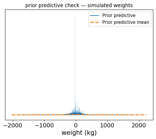
So the results of how those priors affect the data are shown. These results show a very chaotic spread, with negative values well within the realm of possibility, or values of +300 kg being quite plausible too.

This is the model saying “sure, a person could weigh -50 kg or 700 kg, why not?

Exactly the kind of situation where a prior predictive check will save you the embarrassment.

Refining our priors (making an educated guess)

Now that we’ve seen how wild the prior predictive distribution can get with vague priors, let’s try something better.

We’ll use some simple, real-world intuition:

Most adult humans weigh somewhere around 60-90 kg (subject to debate, but this is the assumption we make), so let’s center our intercept around 70-75 kg.
We expect taller people to weight more. A one standard deviation increase in height might correspond to a 5-10 kg increase in weight (again, we make this assumption or educated guess based on our gut, still valid), so we’ll center the slope around 6.
We’ll also pick a more reasonable prior for the standard deviation sigma, reflecting typical variability in weight, not hundreds of kg.

Those priors are still flexible. We’re not being overly confident here, but we are still respecting real-world ranges.

with pm.Model() as better_model:
    intercept = pm.Normal("intercept", mu=72, sigma=10)
    slope = pm.Normal("slope", mu=6, sigma=3)
    sigma = pm.Exponential("sigma", 1)

    mu = intercept + slope * height_scaled
    weight = pm.Normal("weight", mu=mu, sigma=sigma, observed=weight_obs)

    better_prior_pred = pm.sample_prior_predictive(draws=1000)

# visualize the results
az.style.use("default")
az.plot_ppc(better_prior_pred, group="prior", kind="kde", data_pairs={"weight": "weight"})
plt.title("prior predictive check — refined priors")
plt.xlabel("weight (kg)")
plt.show()

Sampling: [intercept, sigma, slope, weight]

png

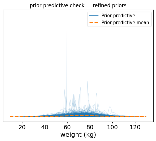
Now you should see a clean distribution of predicted weights, mostly falling between 40 and 110 for the most part (I’m just eyeballing here). This is far more reasonable and aligns with what we expect for adult weight.

The last prior predictive check looked pretty good. Our model was generating realistic weights. But we can take it one step further.

Now that we’ve seren the prior predictive in action, let’s tighten our priors slightly. This isn’t about being overly confident, it’s about acknowledging that we have a pretty good sense of the range we’re expecting.

Our intuition:

Average adult weight is still around 72 kg, but we’re more confident now, so we’ll reduce the standard deviation to 5
A one standard deviation increase in height likely increases weight by about 6 kg, but again, we’ll narrow the standard deviation slightly, maybe to 1.
We’ll keep sigma as-is since our previous setting was reasonable.

These are still not hard constraints, they just express stronger beliefs based on what we’ve already seen and know about the domain.

with pm.Model() as tight_model:
    # more confident (but still flexible) priors
    intercept = pm.Normal("intercept", mu=72, sigma=5)
    slope     = pm.Normal("slope", mu=6, sigma=1)
    sigma     = pm.Exponential("sigma", 1)

    # linear model
    mu = intercept + slope * height_scaled

    # likelihood (we're still not fitting to real data yet!)
    weight = pm.Normal("weight", mu=mu, sigma=sigma, observed=weight_obs)

    # sample from the prior predictive distribution
    tight_prior_pred = pm.sample_prior_predictive(draws=1000)

az.plot_ppc(tight_prior_pred, group="prior", kind="kde", data_pairs={"weight": "weight"})
plt.title("prior predictive check — tight priors")
plt.xlabel("weight (kg)")
plt.show()

Sampling: [intercept, sigma, slope, weight]

png

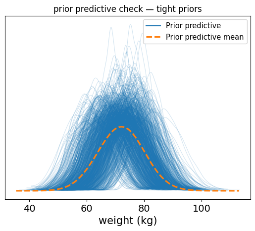
So now we see a cleaner, tighter distribution of plausible weight values, tightly centered around realistic values, with some variability.

This is the kind of prior predictive you want: it reflects your understanding of the world, respects the data scale, and still leaves room for learning from the actual observations

Running inference: let the model see the data

At this point, we’ve checked our priors, refined them, and made sure they produce reasonable simulated data. Now’s it’s time to move from prior to posterior. In other words, to let the model learn from the actual data you have.

We’ll keep the same model structure and priors as in the previous step (the tightened version). We can easily do so by extending the posterior data from inference, into the same data container.

with tight_model:
    # sample from the posterior
    trace = pm.sample(2000, tune=1000)

# plot the posterior
az.plot_posterior(trace, var_names=["intercept", "slope", "sigma"], hdi_prob=0.95)

Initializing NUTS using jitter+adapt_diag...
Multiprocess sampling (4 chains in 4 jobs)
NUTS: [intercept, slope, sigma]



Output()

Sampling 4 chains for 1_000 tune and 2_000 draw iterations (4_000 + 8_000 draws total) took 1 seconds.

png

Sanity check: posterior predictive check

finally, we can check how well our model does after seeing the data by sampling from the posterior predictive distribution.

with tight_model:
    # sample from the posterior predictive distribution
    post_pred = pm.sample_posterior_predictive(trace, var_names=["weight"])

# plot the posterior predictive distribution
az.plot_ppc(post_pred, group="posterior", kind="kde", data_pairs={"weight": "weight"})

Sampling: [weight]



Output()

png

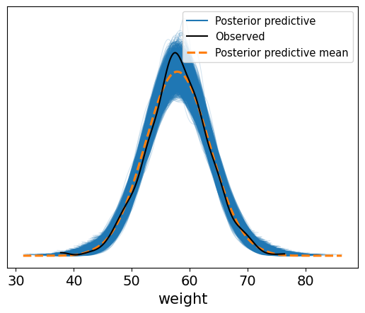
The resulting plot shows how well the model predicts the observed weights. The black line shows the real data, while the blue curves show what our model now thinks is likely.

You’ll notice it’s more concentrated than the prior predictive. That’s the model learning. After seeing the data, our uncertainty about weight has narrowed sifnificantly

This is a nice sanity check that confirms our model is reasonable and captures the data-generating process well.

What did the model learn?

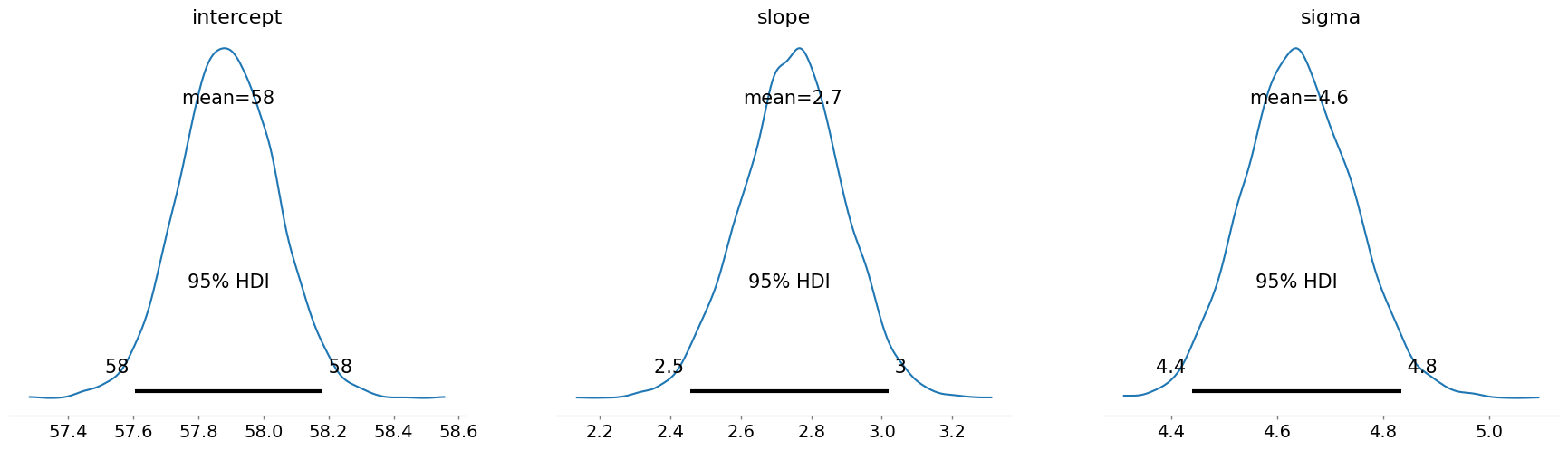
Here is what the posterior tells us:

The intercept (average weight at mean height) is around 58 kg.
The slope is about 2.7 kg per SD of height: so taller people do weight more, but the effect isn’t huge.
The sigma (unexplained variation in weight) is around 4.6 kg, showing there’s still some natural variabilty not captured by height alone.

These estiamtes make sense, and most importantly, they came from priors we were happy with, so we can trust the posterior.

Wrap-up: what we learned about priors

Let’s recap what we did:

We started with vague priors, saw that they produced absurd predictions, and realized that was a problem.
We refined those priors using basic knowledge, and verified our assumptions using prior predictive checks.
Once we were happy, we ran inference, and saw how the model combined our beliefs and data to update our understanding.

Bayesian modeling is not just about plug n’ chug the data. It is about thinking carefully and honestly about what you believe and letting the data update that belief.

The key takeaway: keep in mind where to begin when choosing priors, check them, and don’t be afraid to tweak them. Your model will thank you.

Start with the data¶

So how do you pick a likelihood?¶

So where do priors come in?¶

Choose priors for your parameters¶

What should guide your choice of prior?¶

First: Respect the domain of the parameter¶

Second: Ask yourself what you know¶

Priors matter more when you have less data¶

How do you check if your priors make sense?¶

Check your prior: prior predictive checks¶

What is a prior predictive check?¶

Why is this helpful?¶

A step-by-step prior predictive check¶

Start knowing nothing, or almost nothing¶

Refining our priors (making an educated guess)¶

Final refinement: tighten the priors¶

Running inference: let the model see the data¶

Sanity check: posterior predictive check¶

What did the model learn?¶

Wrap-up: what we learned about priors¶